# Types of EDA
There are four primary types of exploratory data analysis (EDA):
## **1. Univariate non-graphical**
This is the simplest form of data analysis as during this we use just one variable to research the info. The standard goal of univariate non-graphical EDA is to know the underlying sample distribution/ data and make observations about the population. Outlier detection is additionally part of the analysis. The characteristics of population distribution include:
1. **Spread:** Spread is an indicator of what proportion distant from the middle we are to seek out the find the info values. the quality deviation and variance are two useful measures of spread. The variance is that the mean of the square of the individual deviations and therefore the variance is the root of the variance.
2. **Central tendency:** The central tendency or location of distribution has got to do with typical or middle values. The commonly useful measures of central tendency are statistics called mean, median, and sometimes mode during which the foremost common is mean. For skewed distribution or when there’s concern about outliers, the median may be preferred.
3. **Skewness and kurtosis:** Two more useful univariates descriptors are the skewness and kurtosis of the distribution. Skewness is that the measure of asymmetry and kurtosis may be a more subtle measure of peakedness compared to a normal distribution
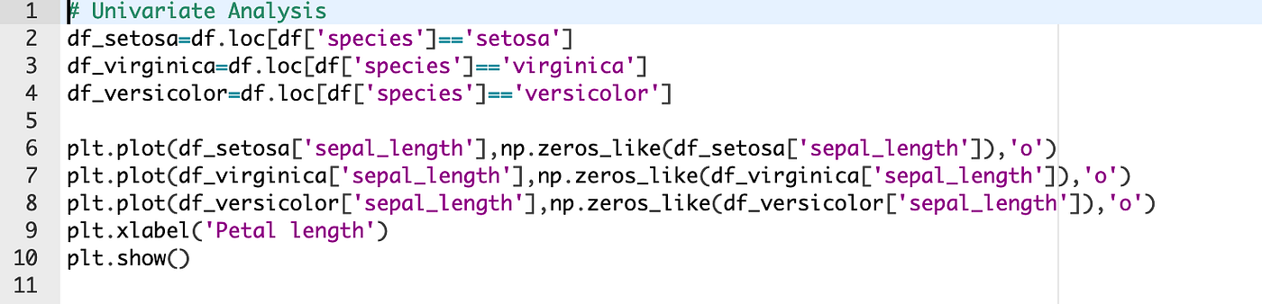
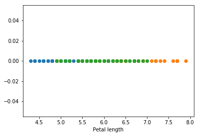
## **2. Univariate graphical**
Univariate analysis is the simplest form of data analysis where the data being analyzed contains only one variable. Since it’s a single variable it doesn’t deal with causes or relationships. The main purpose of univariate analysis is to describe the data and find patterns that exist within it.\
\
You can think of the variable as a category that your data falls into. One example of a variable in univariate analysis might be “age”. Another might be “height”. Univariate analysis would not look at these two variables at the same time, nor would it look at the relationship between them.
Some ways you can describe patterns found in univariate data include looking at mean, mode, median, range, variance, maximum, minimum, quartiles, and standard deviation. Additionally, some ways you may display univariate data include frequency distribution tables, bar charts, histograms, frequency polygons, and pie charts.
Common sorts of univariate graphics are:
1. **Histogram:** The foremost basic graph is a histogram, which may be a barplot during which each bar represents the frequency (count) or proportion (count/total count) of cases for a variety of values. Histograms are one of the simplest ways to quickly learn a lot about your data, including central tendency, spread, modality, shape and outliers.
2. **Stem-and-leaf plots:** An easy substitute for a histogram may be stem-and-leaf plots. It shows all data values and therefore the shape of the distribution.
3. **Boxplots:** Another very useful univariate graphical technique is that the boxplot. Boxplots are excellent at presenting information about central tendency and show robust measures of location and spread also as providing information about symmetry and outliers, although they will be misleading about aspects like multimodality. One among the simplest uses of boxplots is within the sort of side-by-side boxplots.
4. **Quantile-normal plots:** The ultimate univariate graphical EDA technique is that the most intricate. it’s called the quantile-normal or QN plot or more generally the quantile-quantile or QQ plot. it’s wont to see how well a specific sample follows a specific theoretical distribution. It allows detection of non-normality and diagnosis of skewness and kurtosis
* Univariate graphical analysis involves using visual methods to gain a more comprehensive understanding of the data.
* Common techniques used in this type of analysis include:
* **Stem-and-leaf plots**: These plots show all data values and the distribution's shape.
* **Histograms**: They provide a bar plot representation of the frequency or proportion of cases for different value ranges.
* **Box plots**: These graphs display the five-number summary, including the minimum, first quartile, median, third quartile, and maximum values.
## **3. Multivariate non-graphical**
Multivariate non-graphical EDA technique is usually wont to show the connection between two or more variables within the sort of either cross-tabulation or statistics.
For categorical data, an extension of tabulation called cross-tabulation is extremely useful. For 2 variables, cross-tabulation is preferred by making a two-way table with column headings that match the amount of one-variable and row headings that match the amount of the opposite two variables, then filling the counts with all subjects that share an equivalent pair of levels.
For each categorical variable and one quantitative variable, we create statistics for quantitative variables separately for every level of the specific variable then compare the statistics across the amount of categorical variable.
Comparing the means is an off-the-cuff version of ANOVA and comparing medians may be a robust version of one-way ANOVA.
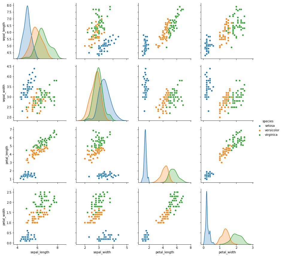
## **4. Multivariate graphical**
Multivariate graphical data uses graphics to display relationships between two or more sets of knowledge. The sole one used commonly may be a grouped barplot with each group representing one level of 1 of the variables and every bar within a gaggle representing the amount of the opposite variable.
Common techniques in this type of analysis include:
1. **Scatterplot:** These plots show the relationship between two variables by plotting data points on a horizontal and vertical axis.
2. **Run chart:** These line graphs display data plotted over time, providing insights into trends and patterns.
3. **Heat map:** Heat maps present data using color to represent values, providing a visual depiction of patterns or variations.
4. **Multivariate chart:** It’s a graphical representation of the relationships between factors and response.
5. **Bubble chart:** It’s a data visualization that displays multiple circles (bubbles) in two-dimensional plot.
[](https://visitorbadge.io/status?path=https%3A%2F%2Fgithub.com%2Fdrshahizan)
---
# Agent Instructions: Querying This Documentation
If you need additional information that is not directly available in this page, you can query the documentation dynamically by asking a question.
Perform an HTTP GET request on the current page URL with the `ask` query parameter:
```
GET https://drshahizan.gitbook.io/eda1/course-content/eda-techniques-and-approaches/types-of-eda.md?ask=
```
The question should be specific, self-contained, and written in natural language.
The response will contain a direct answer to the question and relevant excerpts and sources from the documentation.
Use this mechanism when the answer is not explicitly present in the current page, you need clarification or additional context, or you want to retrieve related documentation sections.